interpretability x retrieval: an emerging field

Interpretability research has spent the last few years opening up large language models, finding features, circuits and steerable directions inside what we used to treat as black boxes. I'm pretty interested in and astonished by that stuff, and I must admit my interest began mostly as admiration for the pursuit itself, decoding the black box as pure science, rather than for practical applications such as AI safety. But in time, seeing the actual practical implications changed that.

Afterwards, as a search engineer, I wondered if these methods are being applied to retrieval models. I was aware of some studies on hubness, theoretical limits etc., but I only recently realised that there is an emerging field working on that question.

I have been reading in this young area for a while, and this essay is my field notes on three papers I liked most for fellow practitioners. Three findings, each explaining something you have probably seen in production, some of them you can already act on.

Relevance Signals are Localised

Let's start with the model family that powers most vector databases, and semantic search applications everyday: the bi-encoder.

A reasonable prior about these models is that relevance lives everywhere and nowhere: tens of millions of weights, each participating a little, none of them meaning anything alone. It turns out this prior is wrong, and it is wrong in a useful way.

In the study that started this whole area, called Axiomatic Causal Interventions for Reverse Engineering Relevance Computation in Neural Retrieval Models (Chen, Merullo and Eickhoff, SIGIR 2024), the researchers took TAS-B, a standard bi-encoder based on DistilBERT, and asked a plain question: when the model rewards term frequency, where does that computation actually happen? (Or does it happen in a specific place at all?)

To answer it, they used a technique commonly used in mechanistic interpretability of LLMs: change one small thing in the input, run the model on both versions, then swap internal activations between the two runs one component at a time, and determine which components move the relevance score. The technique is called activation patching.

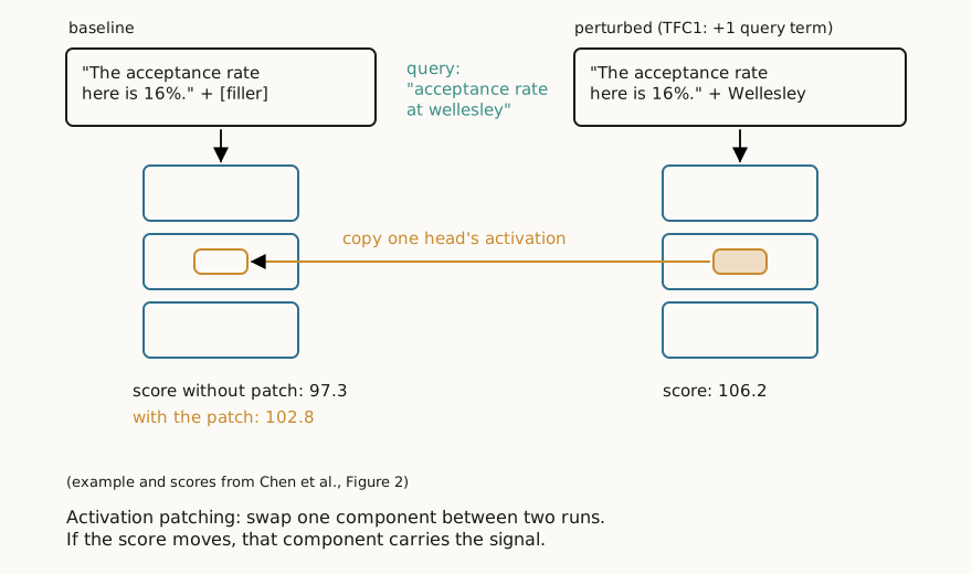
But how do you decide what to change in the input? They take it from axiomatic IR, a line of retrieval theory from the mid-2000s that writes down common-sense rules any good ranking function should obey. For example:

TFC1: If another occurrence of a query term is added, the score should go up.

STMC1: If a term semantically similar to a query term is added, the score should go up.

Think of them like unit tests for ranking functions. The researchers turn a rule into pairs of documents differing in exactly one property, and ask which parts of the model respond to the difference. For term frequency, that means one extra occurrence of a query term, and nothing else changed.

The answer was not "everywhere". Four attention heads carry the relevance signal (0.9, 1.6, 2.3 and 3.8, in layer.head notation), and they do not all do the same job:

• The early ones behave like counters for term frequency. They attend to duplicate occurrences of query terms, literally keeping track of repetition, and the term frequency information is written into those token positions.
• The middle ones behave like composers. They do not attend to duplicates at all, yet silencing them still hurts, and no single token type explains their contribution. The authors' interpretation: the counters write the term frequency signal into the residual stream, and these heads read it and fold it into a broader relevance picture spread across the document.
• And the last two layers are quiet. By then the model has made up its mind, and the relevance information is consolidating into the pooled representation.

And this is not a one-model curiosity. An independent group (Vast, Van Cooten, Soulier and Piwowarski) found the same shape in cross-encoders for reranking: attention heads specialised in matching. Cut the information flow feeding the final representation and nDCG@10 collapses from 0.81 to 0.48, which is exactly what ranking at random scores. That last part matters: the damage is measured in retrieval quality.

So the good news is, the model is not completely a black box, signals have addresses.

Cross-Encoder Rediscovers BM25's Ingredients

One must remember that the point of machine learning models is recognising patterns, and inferring from data utilising these patterns, or functions.

A specific architecture for machine learning, which is called the neural network, is a "universal function approximator", even with a single hidden layer. And these networks are the very basis of modern large language models.

Cross-encoders are a kind of language model that learns to rank search results. Which function might they be approximating?

It's none other than BM25, according to the paper written by Meng Lu, Catherine Chen and Carsten Eickhoff, Pathway to Relevance: How Cross-Encoders Implement a Semantic Variant of BM25.

Before continuing, let's talk about BM25, which is the common standard scoring function for lexical search applications. It builds upon some simple but elegant ideas:

• The more frequent a term of a query in a document, the more relevant the document to that particular query. That part is represented by Term Frequency (TF).
• If that term is rare in all documents (if it is not a word like "the"), it is more valuable. That part is represented by Inverse Document Frequency (IDF).

Up to this point, multiplying TF and IDF gives a basic scoring function, called TF-IDF. But there are two more things to solve:

• Where do we draw the line for term frequency in a document? That part is represented by k₁, the term saturation coefficient.
• A lengthy document will naturally have higher term counts just by being long. That part is represented by b, the length normalisation coefficient.

score(q, d) = Σ_{t ∈ q} IDF(t) · TF(t,d) · (k₁ + 1)TF(t,d) + k₁ · (1 − b + b · |d|/avgdl)

To sum up, term frequency, saturated by k₁, discounted by document length through b, weighted by rarity, summed over the query terms.

BM25 is an elegant idea, but using BM25 directly is not always the best option. It takes only exact words into account. If the query says "car" and the document says "automobile", BM25 finds no match at all. Each term is an atom, per se.

We previously mentioned that neural networks approximate functions. Of course, a function an LLM approximates is very complex to represent, and also opaque. So the authors reach for the unit-test method from the previous finding, in a sharper variant called path patching, and extend the test suite to cover every component of BM25:

STMC1: If a term semantically similar to a query term is added, the score should go up (the semantic sibling of TFC1).

IDF: Rarer terms should count for more.

k₁: Repetition should saturate.

b: Long documents should not win by padding.

(Keep the unit-test framing in mind, we will get back to this.)

It turns out BM25, or better, the concepts that BM25 is supposed to utilise, are represented and used inside cross-encoders. And this should be remembered: nobody told the model to learn them, it was trained on nothing but relevance labels, pairs of queries and documents marked relevant or not. Whatever structure it contains, it emerged.

Several important findings were observed:

• Soft term frequency (term frequency which takes semantically similar terms into account) lives in a set of Matching Heads. These attention heads, sitting in the early and middle layers, light up when a query term appears in the document (their attention also scales with how semantically close a document token is to the query token, the correlation with embedding similarity is around r = 0.50).
• The two BM25 corrections are in there too. Attention to a term jumps at its first occurrence and plateaus with repetition (term saturation, k₁), and it decays as irrelevant content piles up around it (length normalisation, b).
• IDF is represented in one direction of the embedding matrix. This is a finding with more direct practical consequences. If we take the embedding matrix and run SVD on it, the top singular vector closely tracks each token's IDF value (term rarity, correlation around 0.71). It is not distributed across thousands of weights, it is a dial we can use to tune the importances of individual terms or concepts. In the paper, they tried the IDF dial for safety. When the unsafe tokens' component is tuned, 80.4% of 17,537 adversarial samples stopped outranking safe documents, and overall nDCG stayed at 0.9861, a 1.39% drop. That means the model editing is achieved without breaking the ranking performance of the model.
• All of the information above is assembled into a final score at Relevance Scoring Heads, at a late layer. The authors check this by building a plain linear model from just the matching score, the IDF signal, and their product, and it reconstructs the cross-encoder's scores with r = 0.82.
• There is also one genuinely new ingredient BM25 never had: Query Contextualization Heads, that redistribute matching score across query terms according to IDF. BM25 treats every query term as an island. The cross-encoder lets important terms borrow attention from unimportant ones, and that, more than the soft matching, is the semantic variant part.
• They fine-tuned only the embedding matrix for domain adaptation, and it roughly matched full fine-tuning on a small BEIR dataset. It's applied on one dataset with three seeds, but if it holds up, that is a much cheaper adaptation path than alternatives.

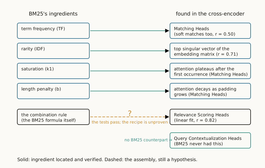
"Implements BM25" is a stronger claim than what the evidence shows. Remember the unit tests: they are design goals, and a whole family of scoring functions passes them (BM25, but also TF-IDF, PL2 and language-model scoring). Passing the tests tells you which family a function belongs to, not which member it is. And at the same time, something better than "it is BM25" is happening: the cross-encoder achieves what BM25 was designed to achieve. Like in the famous quote of Theodore Levitt: "People don't want a quarter-inch drill; they want a quarter-inch hole".

A Dense Model Knows more than a Dot Product can Show

How much can a single vector actually hold?

Every dense retrieval system makes the same bet: that the meaning of a whole document and a query can be compressed into one point in a high-dimensional space, and the relevance between a query and document can be measured as the closeness of two points representing them. It works surprisingly well. But "surprisingly well" is not "always".

Before continuing, let's talk about a finding. In On the Theoretical Limitations of Embedding-Based Retrieval, Weller and colleagues formally proved that for any fixed embedding dimension, there are patterns of relevance that no single-vector system can express. Which documents must match which queries, as a pattern, can exceed what the geometry of d dimensions can realize, no matter how the vectors are placed and no matter how clever the training was.

They built a benchmark called LIMIT that instantiates the worst case using deliberately trivial queries, and state-of-the-art embedding models fail on it badly. The cleanest part of their argument does not even involve a model: optimise the document vectors directly against the test set, with no encoder and no language in the way, and past a critical corpus size the geometry still cannot satisfy all the combinations. The queries are simple enough that the failures look absurd, and that is the point: the difficulty is combinatorial, not linguistic.

So there is a theoretical ceiling that cannot be surpassed by scaling or better training, which makes what comes next much stranger.

Contriever, a standard dense retriever, scores an extremely low 0.053 Recall@100 on LIMIT, as expected. Clavié and colleagues did something interesting: they trained a sparse autoencoder on frozen representations of the model.

Before continuing, I must talk about sparse autoencoders (SAEs) a bit; they became one of the most important tools of modern interpretability. The problem they try to solve is this: in a dense vector, individual dimensions mean nothing on their own, as we can expect. The model needs to represent far more concepts than it has dimensions, so every dimension ends up participating in many unrelated things at once (the phenomenon is called superposition). Dimension 200 of your embedding is not "cars" or "finance". It is a little bit of everything.

The sparse autoencoder solves this. It is a small network trained on the vectors of the original model, and it makes two moves at once:

Its encoder rewrites each dense vector in a much wider space, tens of thousands of dimensions instead of hundreds, under a strict constraint: only a handful of dimensions are allowed to be non-zero for any given input (the sparse part comes here). Its decoder must then reconstruct the original vector from those few active dimensions alone. Squeezed between width and sparsity, the network has only one good option: make each dimension specialise. You can think of it as learning a large dictionary of concepts, and then being forced to describe every vector using only a few words from that dictionary. And the dictionary is inspectable, what you can find is very often a recognisable concept: a single word, a cluster of synonyms, a topic.

The dictionary Clavié and colleagues got turned out to be a vocabulary, which has a usage following a Zipfian distribution (they measure an exponent of about 1.02, almost exactly like natural language). Roughly a third of the features are single surface forms, a tenth are synonym clusters, and over half are broad topical concepts.

And a vocabulary is something you can put in an inverted index. So they were able to score it with plain BM25. The result is 0.729 Recall@100 on LIMIT this time, which is an enormous improvement from the original 0.053.

The theoretical ceiling did not move, because it cannot. What moved is our understanding of where it applies: the bound binds the scoring mechanism, not the representation.

By the way, there is a control experiment that gives further insight: if we run the same SAE on plain BERT before any retrieval training, no retrieval-friendly vocabulary appears. Contrastive training matters here. In the previous finding, the surprise was what grew inside the model. Here, the surprise is what was already inside.

(For completeness about the lineage: this line of work did not start there. Kang, Wang and Xiong had already shown that SAE features on retrieval embeddings can be identified and manipulated to steer rankings. It is a short paper and reads like a proof of concept, but it opened the door the Latent Terms work walked through.)

Worth knowing as you weigh it: this is industry research, from a retrieval company called Mixedbread with academic co-authors, and it is a preprint, not yet peer reviewed.

Two questions remain genuinely open:

• SAE features are known to vary between training runs, so how stable this vocabulary is remains to be shown.
• The SAE itself is trained on a corpus, so how much of that 14x jump is signal recovered from the retriever versus information added by the SAE's own training is a fair question.

What does this mean in practice? Your dense model encodes signal your scoring function cannot express, and sparse methods recover part of it. Hybrid is not a workaround. It is an extraction. And there is early work building the next step directly, using learned sparse vocabularies of latents as the index itself.

What You Can Do With This

So what does all this change in practice?

Usable right now:

• Targeted model editing with a measured cost. The IDF dial from the second finding is real: downweighting chosen tokens mitigated 80% of adversarial rankings at a 1.39% nDCG cost. One model, one dataset, and the authors call it preliminary themselves, but the class of intervention now demonstrably exists. If you run a reranker and fight spam or unsafe content, this is worth an experiment.
• Diagnosis. The patching toolkit is public (the MechIR library, and the field's tutorial ships a runnable notebook). Which relevance signals your model actually computes, and where they live, is becoming an answerable question, at least for the model families these tools support.
• An argument you already needed: hybrid retrieval is principled, not a hack. The third finding is the citation.

Promising:

• Embedding-matrix-only fine-tuning for domain adaptation.

Not yet:

• Steering production rankings through SAE latents. The features are real, but their stability across training runs is an open question, and I have not seen any of this shown surviving contact with production traffic.
• Per-query explanations at serving time. Everything above is offline analysis.

One more honest note. The researchers themselves worry that this field produces explanations without actionable insights; it is the stated concern of their own workshop. Reading their papers as a practitioner, I think the nearer risk is the opposite: the actionable parts exist, and practitioners simply have not noticed them yet. The gap between a cool finding and a shipped intervention is exactly the gap people like us are paid to close.

Interpretability research on dense retrievers has produced genuinely cool findings, they explain things we have all seen in production, and some of them can already improve the systems we run.