representational convergence is not one thing - part 2
Prelude
Part 1 ended at what looked like a conclusion and was actually a question.
The three macro papers (The Platonic Representation Hypothesis, Back into Plato's Cave, and Revisiting the PRH: An Aristotelian View) together pushed the field toward a careful claim: when two neural networks trained differently do agree, what they agree on is something like a neighbourhood graph.
The conclusion of the Aristotelian view is that what "converges" is who is near whom. Not how far apart things are, not the coordinates of any particular point, not the global shape of the cloud. The conclusion/synthesis was that convergence, where it happens, is relational and topological rather than geometric.
That conclusion was the right place to stop a first essay, but of course it was not the right place to stop thinking (I found myself here just because of one particular paper I will talk about anyway!)
Because a neighbourhood is not a self-evident object. A neighbourhood is a set of "near" relations. Near in what space? Built out of what? When a language model represents the concept Monday, or seven, or King, what is the unit of that representation? A vector? A direction? A subspace? A circle? Something I do not yet know a word for?
That is the question Part 2 is about, although it could be safe to say that it now has a clear shape, I would like to keep this open, and hopefully do some hands-on experiments.
Nevertheless, there are a handful of papers that have made progress on it in the right order: The Linear Representation Hypothesis (Park, Choe & Veitch, 2024), The Geometry of Categorical and Hierarchical Concepts (Park, Choe, Jiang & Veitch, 2024), Not All Language Model Features Are One-Dimensionally Linear (Engels et al., 2024), Language Models Use Trigonometry to Do Addition (Kantamneni & Tegmark, 2025), Arithmetic in the Wild: Llama Uses Base-10 Addition to Reason About Cyclic Concepts (Feucht et al., 2026), Emergent World Representations (Li et al., 2023), and Convergent Evolution: How Different Language Models Learn Similar Number Representations (Fu, Zhou, Belkin, Sharan & Jia, 2026).
Part 1 had a Hegelian shape: thesis, antithesis, synthesis. Part 2 does not. Each paper here sharpens the previous paper's answer by showing that the previous paper's answer was incomplete in a specific way. And needless to say, these papers are not exactly on representational convergence as in Part 1, but about representation itself on LLMs.
Concepts can be lines, but only in a particular geometry.
Some concepts are families, polytopes built from those lines.
Some cannot be lines at all, because their value-space wraps around.
Some are a line and several circles braided into one curve, and the model computes by turning it.
Some geometry the model shows you is not the geometry it computes with: it answers a question about months by borrowing a base-10 adder and wrapping the result, so the circle you probe is a costume, not the machine. The model pretends to do things in a more elegant way, if I force the analogies.
Some internal structures the model genuinely uses, which allows editing to change the behaviour.
And in the last paper, the spectral signature of a representation turns out to be a much weaker thing than I would have guessed, present in essentially every model, in a way that does not by itself imply the structure is being used. (Funnily, the title of the paper that sent me toward all the others actually matches my vague expectations.)
Each step is more a refinement than a refutation.
By the end I won't have defended a grand position so much as circled one. Reading these papers in sequence, the possibility I keep coming back to is that meaning in these systems is less a coordinate than a relational constraint, a pattern that holds while other things change, of which lines, circles and helices are passing realisations. I don't think this walk settles that, and I'd rather keep it open.
What it does show, concretely, is smaller and sturdier: that "a concept is there," "you can read it," and "the model computes with it" are three different things, and any claim about convergence has to say which it means.
Lines: the Linear Representation Hypothesis
The first paper is the one with the cleanest version, and became very popular among people working on embeddings.
The story most people carry is the one descended from Mikolov's word2vec work: high-level concepts live as directions in activation space. For example, add a male-to-female vector to king and you get something close to queen, add a positive-to-negative vector to a sentiment representation and you flip the sign or more interestingly, a "speak in French" vector to a context embedding and the model writes in French. Linear probes can read off attributes and steering vectors can change behaviour. It works often enough that nobody quite knows how seriously to take it as a theory. (I was astonished when I had first heard about the word2vec examples while I was a junior data scientist!)
The Linear Representation Hypothesis and the Geometry of Large Language Models (Park, Choe & Veitch, 2024) is a rigorous attempt to ask what this actually means and when it holds.
Three meanings of "linear"
The first move is to think about what concepts are linear directions really means. That statement actually does three different jobs in the literature, and these jobs are not interchangeable.
Assume γ(y) is the model's output vector for a token y and λ(x) is the vector for the input context x.
- Subspace. A concept corresponds to a particular direction γW, and counterfactual word pairs differ along it (like in the famous word2vec example):
γ(king) − γ(man) + γ(woman) ≈ γ(queen)
i.e. γ(king) − γ(queen) ≈ γ(man) − γ(woman) - Measurement. Fix a counterfactual pair (a word in French and its English translation for example) and ask which the context prefers. The log-odds between just those two (conditional on the next token being one of them) is linear in λ(x), along the concept direction:
logit P(French | French or English, x) = γW⊤λ(x)
- Intervention. Adding a different vector λW to the context shifts the output in a controlled way:
λ(x) ↦ λ(x) + α λW, and P(French | x) rises with α
These three live in different spaces: subspace and measurement both are on the output-space direction γW, while intervention happens in the model's input along a separate vector λW. The relationship between the two is not given by the model's training, they need not even point the same way, and pretending it is gives you sloppy claims that conflate three distinct things.
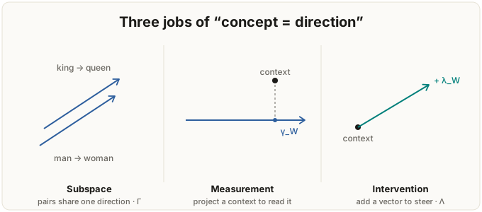
That output/input split has an important second reading, and it is the one that ends up organising the rest of this essay.
The first two notions, subspace and measurement are observational claims about what is present in a representation:
Subspace says a direction exists, measurement says a passive linear probe can read the value of a concept off it with the model untouched.
The third, intervention is causal. Intervention is a write: you add the vector to the final context representation λ(x) (the last hidden state, the one the unembedding turns into a distribution) and ask whether the output actually moves. In the LRH's last-layer setting it provably does; the harder question, for a direction buried in some intermediate layer, is whether the model reads it downstream at all (whether the model uses it at all), and that is the question we seek answers for.
And presence does not imply use. A direction can sit in the geometry, be cleanly decodable, and still be epiphenomenal1: present and readable, but not used, so that steering along it changes nothing. (The standard way to catch this is the ablation test of Amnesic Probing (Elazar et al., 2021): remove the feature from the representation and watch whether behaviour changes, precisely because being able to read it off does not prove the model uses it.)
The direction that best separates the counterfactual pairs need not be the one that best steers the output: a probe can lock onto a feature that merely correlates with the concept in the data rather than the one the model acts on. So the three meanings are not only three jobs in different spaces, they are three claims of increasing strength: the concept is a direction, you can read the direction, the model uses the direction. Within the LRH's own last-layer setup, the first two are not independent: the subspace direction is the probe direction (the softmax identity above), and the embedding representation provably steers; what can come apart on its own is the step up to use in the general case, a direction sitting in some intermediate layer that no downstream computation reads. Only that last step is about the machine rather than the map. I am flagging the seam early because the whole essay eventually splits along it: here, in the tidy word2vec picture, the gap between signal present and signal used is small enough to ignore; by the last paper it is the entire result.
This is the kind of clarification that sounds pedantic until you realise how much interpretability work gets harder when it is missing.
The gauge problem and the causal inner product
One of the important contributions of this paper is what comes next, and it is the part with the most to say about how we use embeddings in practice. Language modelling (like in most deep learning applications) ends in a dot product. The model scores each candidate next token y by pairing the context vector λ(x) with the token's unembedding vector γ(y) and softmaxing the result:
P(y | x) ∝ exp( λ(x)⊤ γ(y) )
This scoring has a hidden symmetry. Take any invertible matrix A, stretch and skew the context vectors one way and the token vectors the opposite way,
λ → A−⊤λ, γ → Aγ + β
and every dot product, and therefore every prediction the model makes, comes out exactly the same.
What this means is that the ordinary Euclidean inner product on activations, the plain dot product behind cosine similarity, is not something the model handed us. It is a coordinate system we picked. Two people analysing the same model under two different choices will report two different answers about which concepts are "orthogonal," which are "close," which "align," and the model has no opinion about who is right. It never committed to a canonical way of measuring.
This is, dressed up in the language of representation learning, a gauge problem, and the physics is worth unpacking, because the analogy is close enough to do real work.
Think about the potential energy of a book on a shelf, U = mgh. To use that formula you have to measure the height h, and to measure height you first have to decide where h = 0: the floor, the desk, sea level. That choice is completely free, because nothing you can observe depends on it. Shift the zero by any constant, h → h + C, and every energy changes by the same mgC, which cancels the instant you take a difference. The book releases exactly the same energy falling from shelf to desk whichever zero you chose. Only differences are physical in that case, the absolute number is arbitrary. (Voltage is the same story, which is why a bird on a high-voltage wire is unharmed: it bridges no difference, so the huge absolute voltage never touches it.) Physicists call that free choice a gauge, and the quantities that survive every choice of it, the differences, are the real content.
The softmax symmetry is exactly this kind of fact. The model's predictions are the gauge-invariant part: they do not move when you apply A. The coordinate system you lay over the activations, the thing that decides whether two concept directions count as "orthogonal" or "aligned," is like the choice of where zero height sits: a convention you added on top, that the model never signed off on.
So when someone reports a cosine similarity between two embeddings, part of that number is real structure and part of it is the gauge they happened to pick, and nothing in the raw activations tells you the ratio.
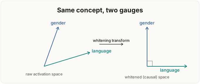
So, for the LRH, the question becomes: what is the right gauge for thinking about concept directions? The paper's answer is the causal inner product.
The intuition: pick the inner product such that causally separable concepts become orthogonal. Two concepts are causally separable if you can vary one without varying the other, male/female and English/French, say, but not English/French and English/Russian: a single word cannot be made French-rather-than-English and Russian-rather-than-English at the same time. Under the right gauge, semantically unrelated concepts should not interfere with each other.
The paper proves that under a few assumptions (that a causal inner product exists at all, that d mutually separable concept directions span the space), the causal inner product has a convenient explicit form. To be precise, the paper characterises a whole family of causal inner products; what follows is the one member of that family (the D = I choice) that the experiments actually use:
M = Cov(γ)−1
In words: whiten the unembedding vectors by their covariance. Whitening is the z-score every data scientist already knows, generalised from one feature to a whole space. Standardising one feature (subtract the mean, divide by the standard deviation) puts it on a scale where a distance of one means one standard deviation (whatever the original units were). Whitening does that in every direction at once, and adds what a per-feature z-score cannot, rotating away the correlations between directions so all are balanced. (The name is borrowed from white noise, which carries equal power in every direction.)
Geometrically, the raw unembedding cloud is a tilted, stretched ellipsoid; whitening squashes the wide directions and stretches the thin ones until it is a round sphere. That sphere is the basis where the covariance is the identity, and there, unlike in the raw space, the plain dot product behind cosine similarity measures what you think it does.
And choosing this gauge does something I find genuinely satisfying: it closes the gap I opened back in the three-meanings section. Remember that the read direction (the one a probe projects onto, γW) and the write direction (the one you add to steer, λW) lived in different spaces and did not have to point the same way. The whitening is exactly the move that lines them up. Written out, the steering vector is λW = Cov(γ)−1γW: the read direction γW, run through the same inverse-covariance. In the model's raw coordinates these are still two different arrows: λW does not point the same way as γW. But the causal inner product is precisely a change of gauge (formally a Riesz map between the two spaces) and in the whitened representation it defines, where separable concepts are orthogonal, the two coincide.
So now, the three meanings (subspace, measurement, intervention) do not merely coexist under the right gauge, they collapse onto a single object. That collapse is the real content of the result and it is the strongest form the linear-representation claim takes in the paper.
This is a refinement that almost rescues the "folk LRH". It says: the linear direction picture works, you just have to choose the right inner product before you start drawing lines.
Two cautions keep this honest, and both matter later. The gauge is not unique: orthogonality of separable concepts pins it down only up to a handful of leftover degrees of freedom, so Cov(γ)−1 is a principled choice rather than the canonical one, and all of it lives in the model's last layer, the unembedding, not in the intermediate computation where the work actually happens. The picture is not even universal among the concepts the paper itself tests: most counterfactual pairs fall cleanly onto a shared direction, but at least one, thing⇒part, shows no linear direction at all. The line, even in the perfect gauge, is a claim that holds often and approximately: not always, and not exactly (I personally find "not exactly" things very useful sometimes, maybe more useful than "exactly"s in some cases. I will talk about this later, maybe not in this blog post.)
There is also a ceiling on the trick that has nothing to do with any single concept, and here I am extrapolating past the paper, so take this as my reading rather than its result:
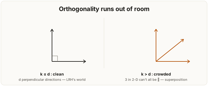
Whitening can buy you orthogonality, but only so much of it: the LRH only asks causally separable concepts to be orthogonal, and a d-dimensional space holds at most d mutually perpendicular directions. A gauge cannot conjure more than the room allows. Below that ceiling (few enough concepts that they can be separated cleanly) you at least have the room the LRH needs, though room is necessary and not sufficient: you still need the concepts to be linearly represented, cleanly paired by counterfactuals, and causally separable in the paper's own sense. Above it (more features than dimensions, which is the regime most people believe real language models actually inhabit) no choice of gauge can keep them all apart, and a model may pack features almost orthogonally and live with the interference.
That second regime has its own name, superposition, and its own literature (Elhage et al.'s Toy Models of Superposition, 2022, is the canonical reference); what I want to borrow here is only the shape of the boundary. The causal inner product is what concepts are orthogonal costs when you can afford it. Superposition is what happens when you cannot. Read this way, the LRH is not the general theory of concept geometry: it is the luxury edition, valid while the concepts you care about are few enough to be kept tidy. Capacity is one way the line picture runs out of room, by crowding. There is another, and it has nothing to do with how many concepts there are.
Categories: when a concept is a family
The line picture has an obvious next question: King might be a direction, but what about mammal, which is not one thing but a whole family (dog, cat, whale, bat)? And what about the fact that mammal sits inside animal, which sits inside living thing? A single direction cannot hold a category and its place in a hierarchy at once.
The Geometry of Categorical and Hierarchical Concepts in Large Language Models (Park, Choe, Jiang & Veitch, 2024) is the same group's follow-up to the LRH, and it answers this with more linear algebra. It needs one new ingredient first: a magnitude. An LRH direction has none by definition, and the paper shows a clean feature comes with a natural one: in the ideal case every mammal word (dog, cat, whale) sits at the same height along the "mammal" vector, non-mammals at zero, and that shared height is its length, turning a bare direction into an actual point. (Their phrase: "cat is exactly as much a mammal as dog." Every member at the same height is what makes the vector mean mammal-ness.)
With real points in hand, a binary concept is still a single arrow. But a categorical concept such as a set of mutually exclusive options like {mammal, bird, reptile, fish} becomes a polytope (and for a clean category a simplex). The member-points are its corners, a triangle or a higher-dimensional tetrahedron, one per option, and the old binary contrasts are its edges.
The hierarchy between concepts is encoded by orthogonality. For example, the direction that separates animals from non-animals is perpendicular, measured in the same whitened geometry the Lines section relied on, to the directions that sort animals into their kinds, so the model can move down the tree without disturbing where it sits higher up. Complex concepts become polytopes, simplices stacked at right angles along the hierarchy.
On Gemma and LLaMA-3 they estimate the vectors for 957 WordNet concepts and confirm the hierarchy is orthogonal there, and the orthogonality survives a sharp control: swap a concept's true parent for a random one and the right angle vanishes, so it is real semantic structure and not the near-orthogonality any two vectors already share in high dimensions. (This is all the final-layer, softmax geometry; how the internal layers arrange these concepts is left open.)
This is still a linearity in the LRH's sense, since every piece is a direction or a flat arrangement of directions, but it is no longer a story about single directions. A category is the convex hull of its members, a hierarchy is a tower of orthogonal hulls.
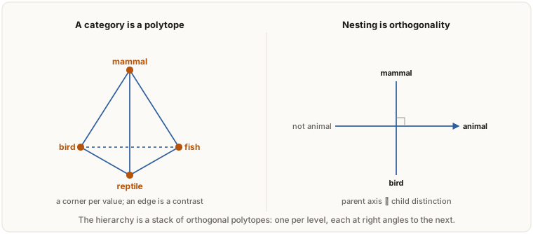
Left: a category is a polytope, a simplex in the clean case, one corner per mutually-exclusive value, with the old contrasts as its edges.
Right: a parent concept sits at a right angle to the distinctions among its children, so the whole hierarchy is a stack of orthogonal simplices.
The geometry is richer than a line and still flat, still made of straight pieces. Which sets up the question the next paper answers with a no: does every concept reduce to straight pieces?
Circles: when concepts can't be lines
Not All Language Model Features Are One-Dimensionally Linear (Engels, Michaud, Liao, Gurnee, Tegmark, 2024; ICLR 2025) starts from a very concrete observation that, in retrospect, is obvious.
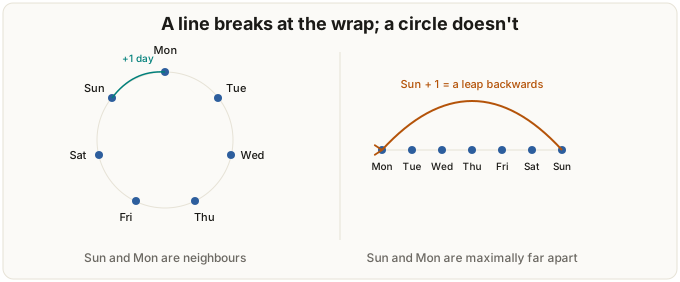
Suppose you wanted a language model to represent the days of the week. You could assign Monday to position 1, Tuesday to 2, and so on up to Sunday at 7. Clean and linear.
This representation has a problem: it gets Sunday + 1 = Monday wrong. On a line, Sunday is far from Monday. In actual semantics, Sunday is right next to Monday. The cycle wraps and represents this accurately, but the line does not.
So, the natural representation for it is a circle. If you place the seven days on the vertices of a regular heptagon, the distance from Sunday to Monday is the same as the distance from Monday to Tuesday. The cyclic structure of the value space is encoded in the structure of the representation.
This paper asks two questions, and answers both:
- Do pretrained language models actually represent things like days, months, and years as circles?
- Are those circles actually used in computation/inference, or are they just cool visualisable artefacts?
The answer to both is yes! (The alternative would be extremely boring.)
In GPT-2-small and Mistral-7B, sparse-autoencoder analysis turns up clean circular representations: a heptagon for days of the week and a dodecagon for months (and, in GPT-2, a coloured spiral for years of the 20th century). And when you intervene on the circular subspace in Mistral-7B and Llama-3-8B (rotating the days-circle and patching it back in), the model's predicted next token follows the rotation. Two days from Monday is Wednesday becomes Two days from Monday is Saturday when you nudge the circle by the right angle.
The method for finding these circular structures which are obviously not labeled "days of the week" is running a sparse autoencoder over the activations (it rewrites each one as a sparse sum over a big dictionary of feature-directions) and then clustering the dictionary. The twist that makes this work: a circle does not show up as two dictionary features (an x-axis and a y-axis). Reconstructing a point (cos θ, sin θ) from two axes fires both at once, and the sparsity penalty punishes that, so the autoencoder instead learns many features pointing at different spokes of the ring, each firing for one small arc. Those many spoke-like elements all span the same plane, so they link into one cluster (adjacent spokes overlap, and the ring connects through that chain). That cluster is a beautiful circle.
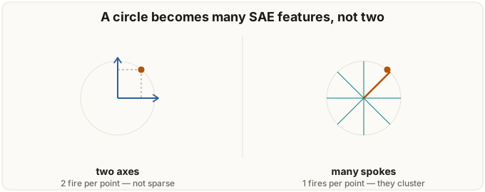
One caution that doubles as this essay's spine: presence is not use. The causal half of that "yes" (intervening on the circle works) is demonstrated for Mistral and Llama. But GPT-2 has the same clean circles and still gets trivial accuracy on the day and month tasks (8 of 49 on weekdays, 10 of 144 on months): the structure is there, and the model simply does not compute with it.
It is important to be careful about what this paper does and does not say. It specifically challenges the first half of the LRH (the assumption that all representations are one-dimensional) and not the second half, which says that hidden states decompose as sparse sums of features. (The refinement is local.) Most features can still be small subspaces; some of those subspaces are 1-D directions and some are not.
Irreducibility
The deep claim of the paper is that these circles are irreducible. You cannot decompose them into independent linear features. The two coordinates of a circle in ℝ² are not statistically independent: they are constrained by x² + y² = 1. No rotation of the basis makes them independent. No projection onto a single direction recovers them.
Independence is only half the test, though. A feature is also reducible if it is a mixture: several lower-dimensional pieces that never co-occur, like a one-hot encoding of "which day" with exactly one slot on at a time. The circle of days is not that either: its seven points all lie in one shared 2-D plane, arranged around a ring, rather than on separate axes the way disjoint one-hot states would. The observed ring-like distribution scores as non-mixture under their test. (Mistral-7B additionally fills the ring in continuously, placing very-early-Monday between days, but irreducibility does not need that continuity; the inferred circle is connected even where the observed token cloud is just vertices.) Irreducible means it escapes both routes at once: not separable into independent parts, and not a mixture of disjoint ones.
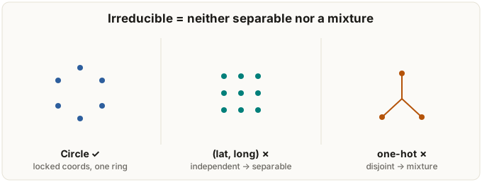
This is where the LRH gauge story stops being enough. There is no choice of inner product that turns a circle into a line. Structure beats geometry: the days of the week carry a finite cyclic order (ℤ/7ℤ), which the model realises geometrically as a circle. (Seven points have no topology worth the name; it is the cyclic order, the +1 wrap, that a straight line gets wrong.) Computing the wrap correctly (Sunday + 1 = Monday) means honouring that cyclic relation somehow; what the paper shows is that these models do it with a circle, not that every adequate representation must. No gauge can bend a straight line into a loop.
(The Engels paper's reducibility test is itself worth a moment: it formalises both escape routes, separability (can the coordinates be made independent by some rotation) and mixture (do the pieces fail to co-occur), as statistical conditions and tests them. The conditions are the right ones: meaningfully sharper than "the variance in some direction is small." The separability half is the old disentanglement goal, independent factors of variation, chased at least since Higgins et al. tried to define it (2018); Engels turns that loose aspiration into a concrete test.)
The value space's structure calls for a particular shape in the representation. A straight line is the special case, the one where the value space is itself a line, not the only one.
Two honest caveats though:
First, the irreducibility tests are statistical, not causal: they describe the shape of a feature's value distribution, not whether the model uses it, which is exactly why the intervention experiments are a separate and necessary step.
Second, the authors are candid that they found surprisingly few clean multi-dimensional features, and do not know whether such features are genuinely rare, mostly higher than two-dimensional, or simply hard for their clustering to surface. So the headline is not models are full of circles. It is narrower and truer: the line is not the only option, and for cyclic concepts it is the wrong one.
The picture sharpens. Some features in language models live in low-dimensional manifolds inside the activation space (the residual stream), not the embedding space proper. They are 2-D rings for cyclic concepts, and collapse to a single direction for binary ones (where the LRH's direction story works in the right gauge). The geometry is whatever the value space demands.
And we are starting to know why the value space gets to demand a shape. A 2026 paper by Karkada and colleagues proves that when a concept's contexts carry a translation symmetry, when how often two values co-occur depends only on how far apart they are and not on where they sit, the embedding that fits those statistics is forced into the matching geometry: periodic values (months, days) onto a circle, non-periodic ones (years) onto a rippling line. The circle is not a lucky find. It is what the data's symmetry compels. A companion result, Modell, Rubin-Delanchy and Whiteley's The Origins of Representation Manifolds in Large Language Models (2025), works the other side of the question: it gives a theory of how a feature unfolds into a manifold and shows that cosine similarity along it tracks the feature's own intrinsic distances, so the shape is not only compelled but legible, near on the manifold means near in meaning. Hold onto that, because the same co-occurrence-makes-geometry principle comes back, with teeth, in the last section.
But this still leaves something unsaid. What about a concept that needs the line and the circle at once? What about numbers, which carry both a magnitude (how big) and a fistful of cyclic structure (odd or even, the units digit, the wrap at every power of ten), and which are arguably the most heavily structured concept in any language model's training data?
Helices: numbers as a line wound into circles
The next paper takes the line and the circle and does the thing the previous sections only gestured at: it catches a model computing with the geometry.
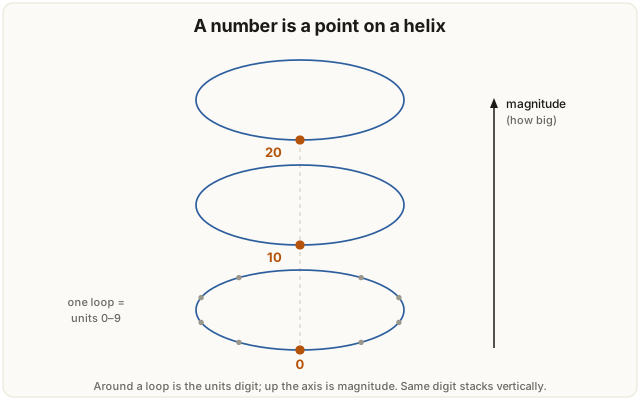
Language Models Use Trigonometry to Do Addition (Kantamneni & Tegmark, 2025) asks how a pretrained model actually adds two numbers, and reverse-engineers the answer down to individual neurons. The representation it finds for a number is a generalised helix: a straight axis that tracks magnitude (bigger numbers sit further along) wound together with circular components at periods 2, 5, 10, and 100.
A clarification worth mentioning, because it is easy to get backwards: the circles are not there because a line cannot add. The authors are explicit that an LLM could do addition on the linear component alone, and they read the helix as the model's way of making addition robust to noise, not a way of making it possible (their appendix conjectures that pure linear addition would be measurably less accurate). The periods, too, are read off the data rather than derived: a Fourier transform of the number representations shows sharp peaks at 2, 5 and 10, and the authors add 100 for its magnitude and a base-10 prior. (That pretrained models add with exactly these base-10 Fourier features had been traced a little earlier by Zhou et al. (2024), who pinned the magnitude work on low-frequency components and the digit work on high-frequency ones.) So the helix is exactly the two shapes this essay built, a magnitude line wound with the periodic features the model actually grew, both genuinely present, but the circles earning their place because the spectrum shows them.
The Clock algorithm
The striking part is that the model does not store the helix and stop. It operates on it. To compute a + b, the authors trace a four-step routine they call the Clock algorithm (after a toy-model precursor in Nanda et al., 2023, named the "Clock" by Zhong et al., 2023): the helices for a and b are laid down on their own tokens, attention heads transport both to the final "=" position, a band of MLP layers reads the a and b helices and builds the helix for a + b, and the last layers read that answer-helix out into a distribution over number tokens.
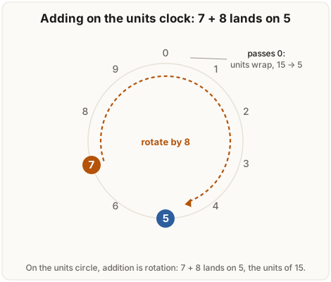
You can picture the middle step as two clocks being added: to get the units of a + b you rotate one clock by the other's angle, and 7 + 8 lands on 5, the units digit of 15. The mechanism the authors propose for that rotation is a trigonometric identity, cos(a+b) = cos a cos b − sin a sin b, which multiplies a coordinate of a by a coordinate of b.
That matters as a clue, because a linear map can scale and add its inputs but cannot multiply two of them together, so the rotation has to come from somewhere nonlinear; and the paper does find the MLPs (layers 14-18) doing most of the work of building the a + b helix, with a few mixed attention heads helping (attention is not purely a transport layer here). But this is exactly where the paper is careful, and so should we be: they cannot isolate the multiplication in the weights. The trig-identity story is a well-motivated hypothesis, matching Nanda's reverse-engineered toy circuit, not a circuit they pinned down.
How strong is the evidence
The evidence is stronger than the previous two sections. They fit each number's representation with the nine-dimensional helix (nine basis functions mapped into the activation space), then patch that fit back into the running model in place of the real activations. The helix, nine numbers, recovers 7.21 of the 8.34 logit-difference you get from patching the full high-dimensional activation. Most of the causal effect of the real representation survives in that nine-dimensional fit. (Worth being precise about where the weight sits: a fit using only the circles, with no line at all, already recovers 6.83, so it is the periodic components doing nearly all of the work and the linear term adding a little.) Either way the point holds, and it is evidence the digit picture never had: not "a probe can read it" but "replace the representation with the helix and the model still computes."
The honest scope. The detailed circuit-and-neuron analysis is on GPT-J (6B); Pythia-6.9B and Llama-3.1-8B get appendix-level replication, and Llama's helix is the least causally implicated of the three (the authors suspect its gated MLPs run a modified routine). Across tasks the helix is strongly causal for addition and subtraction, and for taking a number mod 2, but clearly weaker for multiplication and division. And it is shown for two-digit numbers; three-digit inputs already show a discontinuity, a sign the representation changes with scale. So the claim is precise: for these models, on this range, numbers are helices and the Clock operation works.
Not just neural networks
This is not a quirk of transformers. In 2014 the Nobel Prize in Physiology or Medicine went to O'Keefe and the Mosers for the brain's positioning system, among them the Mosers' grid cells in the entorhinal cortex, neurons whose firing tiles space in a repeating hexagonal lattice; in 2022 Gardner et al. showed that the joint activity of a grid-cell module lives, mathematically, on a torus. A brain encoding where you are and a language model encoding how big a number is have both reached for the same kind of object: a low-dimensional periodic code, a quantity wrapped into circles. The convergence is at the level of what the problem demands, not what the system is made of.
A concept can be a curve that braids the earlier shapes together, a line and several circles, and the model does not merely hold that curve, it computes by moving along it. The unit has grown from a direction (LRH) to a structured stack of directions (Park) to an irreducible circle (No-LRH) to a helix that is genuinely operated on.
Which also plants a question the helix never had to face. Here the geometry we probed and the geometry the model computed with were the same object. The next paper separates them: it finds a model showing you one geometry and computing with another.
Disguises: when the geometry is not the algorithm
It is hard not to conclude the model computes with a geometry when it is found. The helix earned that conclusion, the model really did turn the circles to add. This paper is where that conclusion breaks.
Arithmetic in the Wild: Llama uses Base-10 Addition to Reason About Cyclic Concepts (Feucht et al., 2026) takes the cyclic concepts, months, weekdays, hours, and they are stored exactly as the circle section would predict: months sit on a clean twelve-point circle, December next to January, the mod-12 wrap built into the geometry. So when the model answers what month is six months after August?, the natural guess, the one toy models trained on modular addition vindicate, is that it rotates six steps around the month circle and reads off February.
It does not though. Using distributed alignment search (after Geiger et al.), a relative of the interventions the helix and Othello sections relied on (they patched and edited activations directly, this learns which subspace to patch), the authors localise where the input month and the offset are combined into the answer: sharply, at one MLP in the middle of the network, and at the same place for months, weekdays, hours, and plain a+b. Then they look for the month circle at that location, and it is not there yet. The circle the answer should be computed on cannot be recovered until four to seven layers later, by which point the answer is already forming. The circle is a late re-encoding, the costume the answer is dressed in on its way out, not the machine that produced it.
What produces it is addition, and two interventions nail this. Patch the internal state from a pure 6+8= prompt into a months prompt and the model outputs February, because (6+8) mod 12 = 2; a bare number is enough to make the right month. Patch the other way, from six months after August into a+b=, and the model outputs 14, the raw sum, August being the eighth month. The decisive detail is in that second direction: two prompts that share an answer-month but differ in their pre-wrap sum, a 3 and a 15 that both mean March, patch back as different numbers, 3 and 15. Modular arithmetic is many-to-one and would have thrown that difference away; the model is still holding it, so what it computed was the ordinary linear sum, and it had not yet wrapped. The twelve-ness enters only at the very end.
And the addition is in base ten, not base twelve. Fourier probes trained only on the a+b task recover periods 2, 5, 10, 20, 50, 100, the base-10 fingerprint, and never the 12 that months would call for. Better, those addition-trained probes steer the cyclic tasks: push the internal sum from 7 to 6 and the model shifts toward June instead of July. A control surface learned on arithmetic that drives an unseen month question is what tells you it is one reused machine and not a coincidental lookalike (the steer is a firm nudge on the output distribution, not a clean switch). The machine even has a findable circuit: a sparse set of 28 MLP neurons, about 0.2% of that layer, does almost all of that layer's work on the sum (zero them and the model's addition accuracy falls from 95% to 24%; keep only those 28 and ablate the rest of the layer and it still holds at 86%), clustered by period, with the cyclic tasks drawing their neurons from this same addition set, down to two parity neurons whose only job is to sharpen even against odd.
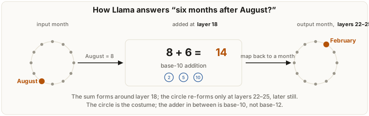
So the month circle is real, it is probeable, and it even reappears late, near where the answer is read out, but it is still not the algorithm. The algorithm is a generic base-10 adder, and the circle is the costume it wears at the door. This is where the optimistic reading, the geometry you can see is the geometry the model uses, takes its first real wound: a structure can be present, even causally downstream, and still be the wrong thing to credit.
(One honest boundary. This is a single model, Llama-3.1-8B, on three cyclic families and forward-offset questions, and the authors deliberately do not explain the final step, how 14 actually becomes February. What they pin down is the localisation and the addition mechanism, and those are enough to break the easy inference from shape to computation.)
Which sets up the two papers left. The next shows that genuine use can be established about as firmly as this kind of question allows, in a case where you can edit the structure and watch the behaviour follow. The last asks how cheap mere presence really is, and answers: very.
World models: structure the model actually uses
Everything so far has been about how a single concept is shaped. This paper changes the question from what shape to is the shape load-bearing, and it does so in a setting about as clean as this question gets.
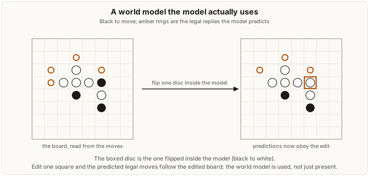
Emergent World Representations (Li et al., 2023) trains a transformer, Othello-GPT, on nothing but sequences of legal Othello moves (no board, no rules, no images, but just strings of moves.) The question is if, from move sequences alone, the model builds an internal model of the board.
It does, and the evidence comes in two strengths. A probe trained on the activations recovers the state of all sixty-four squares, whose piece sits where, even though the model was never shown a board (curiously, at first only a nonlinear probe read it cleanly, a linear one lagged well behind, around 75%). On its own that is only presence, the days-circle problem again: the state is there, but is it used?
The paper closes the gap with intervention. Reach into the activations and nudge them until the model's internal board reads one square flipped, hold the real move history fixed, and the predicted legal moves change to match the edited board.
The sharpest version edits the board into a position no legal game could ever reach: with no training sequences left to imitate, the model still plays that impossible board's legal moves. That rules out mere transcript-matching and pins the board representation as a genuine cause of the move, even if it stops short of proving the model runs an explicit copy of the rules. The world model here is not decoration, unlike the previous case: the model's next move draws on it.
And that early "nonlinear" reading turns out to be a red herring. The linear probe lagged only because it was asked for the wrong coordinate, absolute colour (black or white). Othello-GPT alternates sides every move, and legality depends not on colour but on mine versus yours. This model represents the relative state, and absolute colour is that state XOR'd with whose turn it is, so reading colour back out means undoing an XOR, which a linear probe cannot, hence the colour probe stalls near 75% while the mine/theirs probe sails to 99.5%. Re-probe in the model's own frame, mine / theirs / empty, and the board is cleanly linear (Neel Nanda first found this linear, mine/theirs encoding, with preliminary interventions, in a 2023 note; Hazineh, Zhang and Chiu made it systematic across layers and models).
The world model was linear all along; you simply had to read it in the coordinate the task cares about. That rhymes with the Lines section's right gauge, although it is not the same move: there the fix was a whitening of the space, here it is choosing what to decode. The shared moral is that the structure is only legible in the frame the problem prefers.
This is the cleanest use result in the essay, and the fact that it is not about numbers is the point. The earlier sections kept finding structure inside one heavily-patterned domain. Here the structure is a whole game state, in a domain with no continuous magnitude at all, and the causal test is strikingly direct: change the represented world, change the behaviour. (And, echoing the number papers, the edit bites mostly in the middle layers, and mostly in the earlier part of the game, and fails in the last couple even though the board is most legible at the end, which the follow-up reads as the move being settled mid-network, the late layers holding a finished, legible copy rather than a workspace.)
A representation can be read (a probe finds the board) and used (editing it steers the model), both demonstrated, in a setting clean enough to leave little doubt. Othello-GPT clears the bar the days-circle could not.
Spectra: the same notes, different music
The last paper is the one that started this whole essay series for me. I mentioned the Hacker News discussion in the Part 1 prelude, this is the paper.
Convergent Evolution: How Different Language Models Learn Similar Number Representations (Fu, Zhou, Belkin, Sharan & Jia, 2026) noticed something startling about the periodic structure the helix is built from. (Fu et al. measure it differently from Kantamneni and Tegmark, through the Fourier spectrum of number-token embeddings taken across the integers, rather than a fitted helix, so this is a relative of the helix result, not the identical object.) It is not a Llama thing or a Mistral thing. It is not even a transformer thing. Almost every language-modelling system examined has it.
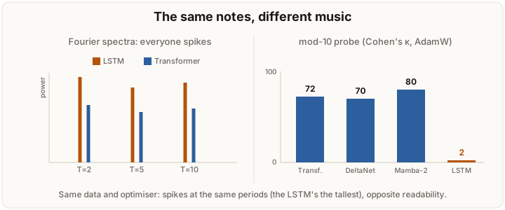
Take the number-token embeddings of the pretrained large language models they survey (GPT-2, GPT-OSS, Llama-3, Llama-4, DeepSeek-V3, Mamba, Falcon-Mamba, xLSTM, Kimi-Linear, even classical word-vector embeddings like GloVe and FastText) and compute the Fourier transform along the integer index. You find clean spectral spikes at periods T = 2, T = 5, T = 10.
The spikes are near-universal across the systems examined. Different architectures (transformers, linear RNNs, LSTMs, classical embeddings), different training data, different training procedures, different tokenisers, and the same dominant periods, 2, 5 and 10, come out of all of them. The magnitudes differ (the LSTM's spikes are actually the largest); what is shared is where the spikes sit.
Even the raw token-frequency distribution of numbers in the training corpus, with no model at all, has the same periodic structure. Round numbers are more frequent; numbers ending in 5 are more frequent than their neighbours; the data has a base-10 fingerprint, and a model that ingests enough natural-language text inherits the fingerprint almost regardless of what else it is doing.
So is this representational convergence? Have they all "discovered" the base-10 modular structure of arithmetic? The temptation to say yes is large, and the paper shows it is unearned: the shared spike does not establish that any system discovered modular structure, and whether that structure is even linearly readable turns out to be selective.
Spectral convergence vs geometric convergence
The vocabulary the paper introduces is a two-tier distinction.
- Spectral convergence: the Fourier spectra of the number embeddings have spikes at the same periods. Almost universal across the systems tested.
- Geometric convergence: the residue classes n mod T are linearly separable in the embedding space. A linear probe can read off "n mod 10" from the embedding. This is more selective: present in some systems, absent in others.
The first means the structure is present in the representation. The second means the structure is functionally usable: that a downstream linear classifier can extract it. One precision worth keeping, since the previous sections set a higher bar: "usable" here means linearly readable, not operated on. The helix paper patched a fitted helix back in and the model still computed; Othello-GPT had a square flipped and changed its move; both are interventional. This paper shows only that the mod-T class can be read off by a linear probe. Present, readable, operated-on are three different rungs, and Convergent Evolution lives on the middle one.
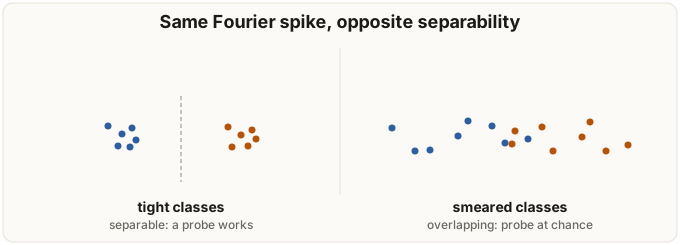
The paper's central theoretical result (Theorem 1) is that spectral spikes are necessary but not sufficient for linear separability. They prove this constructively: you can build embeddings with arbitrarily strong Fourier spikes at period T whose mod-T classes are still no more separable than chance. The mechanism is intuitive once you see it. A Fourier spike at T measures only how far apart the class means are spread (the between-class scatter). It is blind to the spread within each class, which lives at other frequencies and never registers in the period-T power. So you can hold the spike fixed and smear each class outward until the classes overlap: the period-T power is unchanged (the smear lands at other frequencies), the separability collapses. Spectrum tells you the means are far apart. Whether the classes are resolvable depends on the within-class spread the spectrum cannot see.
This sounds abstract until you see the empirical version:
The Fu et al. team trained transformers, linear RNNs, and LSTMs on identical 10-billion-token natural-language data. All three architectures produced number-token embeddings with Fourier spikes at T = 2, 5, 10. The LSTM actually had more prominent spikes than the transformer. Spectral convergence is clearly present in all three.
The mod-T linear probe, on the other hand, splits them apart. The paper reports Cohen's κ, scaled so that 0 is chance and 100 is perfect (raw chance accuracy for mod-10 is only 10%). Holding the optimiser fixed at AdamW, so that only the architecture varies:
- Transformer: κ ≈ 72
- Mamba-2: κ ≈ 80
- Gated DeltaNet: κ ≈ 70
- LSTM: κ ≈ 2 (chance)
The transformer and the linear RNNs read the modular structure off cleanly; the LSTM cannot. (Switching the transformer to the Muon optimiser lifts it to κ ≈ 85, the number usually quoted, but the like-for-like architecture comparison is the AdamW column above.)
The LSTM's Fourier signature looks like modular arithmetic but a linear probe cannot read that structure off its embedding. The signal is present, but not usable.
Two architectures can have near-identical spectral fingerprints and expose the modular structure completely differently to a linear probe, because the bit that matters is not whether the periodic structure exists but whether it stands out from the within-class noise in a direction a linear read can find. (Whether the LSTM could still use that structure by some nonlinear route is a separate question this paper does not test.)
What the usable half feeds on
It is worth being concrete about that alignment. The architecture result above held the data fixed and varied the model. A second experiment does the reverse: hold the architecture fixed and change the data. Resample every number token independently from the corpus-wide frequency distribution (the paper calls this Unigram Replace): each number keeps its overall rate, but every association with its neighbouring words and numbers is destroyed. The Fourier spikes remain all but unchanged; the probe falls to chance.
The spike needs only the marginal statistics: how often each number appears. The readable geometry needs a number's company: what it co-occurs with, both the words around it ("12" near months, inches) and the other numbers near it (sequences, sums). Strip the company and the readable structure dies while the spectrum does not.
This is an old idea in new clothes. "You shall know a word by the company it keeps," J. R. Firth wrote in 1957, and the whole distributional-semantics tradition (and my own journey of embeddings essay) runs on it. Convergent Evolution measures the same principle on numbers: the usable representation of a number is built from its relationships, not from a count of it in isolation. The spike is marginal, the geometry is relational. That contrast is the seed of where this essay is heading.
A musical analogue: modes
This is the analogue I have been holding back through the previous four sections, because it does the most work here.
In Western music, the major scale and its modes (Ionian, Dorian, Phrygian, Lydian, Mixolydian, Aeolian, Locrian) contain exactly the same seven notes. The C major scale and D Dorian have identical pitch content, the same "spectrum" in this loose musical sense. But they sound completely different. They have different tonal centres, different patterns of tension and resolution, different feelings. Major sounds bright. Dorian sounds wistful.
Same notes. Different music.
The notes are the spectrum. The mode is the relational structure that organises the notes into music. Two systems with identical pitch content and different modes produce different output. You cannot recover the mode from the spectrum alone.
There is a sharper version of this. Relative pitch is the ability to hear how notes relate, to recognise a melody in any key, hear chord changes, transpose on the fly: it is holding the relational structure of music. Perfect pitch, naming a note by its absolute frequency, is a separate coordinate-level skill, and many of the greatest musicians do not have it; relative pitch is the one that actually lets you make music. (Even then, pinning down an absolute note from relative hearing needs one reference pitch to anchor it.)
The LSTM in the Convergent Evolution result, in this metaphor, has the notes without the ear for them. The spectral signature is physically present in its embeddings (the raw frequencies are all there), but it has nothing like relative pitch: no relational organisation that would let a linear probe read the residue classes off. The transformer has that organisation; the LSTM has only the easy half, the notes without the hearing that turns them into music.
This is, I think, the single most important framing to take from this paper. Spectral convergence is the easy kind of agreement; it is widely available and it does not by itself say very much. The hard kind of agreement is the readable kind, and it is selective, and it depends on the architecture and the optimiser and the data and the tokeniser all happening to align.
Spectral structure is in essentially every neural representation of numbers examined, largely regardless of architecture. What varies is whether that structure is linearly readable. Whether the within-class noise is small enough, in the right directions, for the signal to stand out.
This is no longer a question about lines or circles or helices. It is a question about whether a particular kind of relational organisation (the one that lets a linear probe read off mod-T residues) is present in the embedding, reachable by a linear probe. And the answer is, sometimes yes, sometimes no, and the difference matters.
And that is where I will stop the walk. Reading these seven papers in sequence left me circling a larger claim: that meaning in these systems is less a coordinate than a relational constraint, a pattern that has to hold while other things change, of which lines, circles and helices are passing realisations. But that is a whole essay of its own, and folding it into the tail of this one did it no favours, so I will make it properly, and separately, next. For now the narrower, hard-won result is enough: convergence is real, but it is relational, and the same shape can be present without being used.
What's next
The series is not closed. There are many papers I explored while writing this blog post, and I stumbled upon many interesting questions.
The papers themselves are the canonical record, and I am very grateful to all the authors who wrote them.
Comments, pushback, and corrections are welcome. This series is my attempt to map a landscape I am still actively exploring, and the map gets sharper with every reader who notices something I have missed.
This is Part 2 of a series on representational convergence. Part 1 is here.
- The word comes from philosophy of mind, where epiphenomenalism (associated with Huxley, 1874) holds that consciousness is a byproduct of brain activity that itself causes nothing: "the steam-whistle which accompanies the work of a locomotive engine is without influence upon its machinery." A direction you can read but that the model never acts on is that whistle. Back to text